In this post, I’m going to use R to scrape Indeed.com for some jobs, then plot the positions of the top jobs on a map, and save that map to disk. We also want to scale the geographic region with a circle whose size is proportional to the number of jobs. If you’re successful, you should see something like this:
To do this, we need these libraries:
library(rvest)
library(httr)
library(stringr)
library(rgdal)
library(leaflet)
library(ggplot2)
library(plyr)
library(mapview)
library(htmlwidgets)
Also to plot the locations of the cities where the jobs are I used the free airport.csv data at: http://ourairports.com/data/
First we’re going to load our airport data:
airports <- read.table(
"C:/workspace/news_scraper/airports.csv",
sep=",", header=T, stringsAsFactors = F, fill=T)
airports$municipality<-toupper(airports$municipality)
We going to make a function that will take a job string that’s in the form of an url parameter. It will download the webpage that’s at that url, and save the page to disk::
download_string=paste("https://www.indeed.com/jobs?q=",job_string,sep="")
download.file(download_string, destfile = "C:/workspace/news_scraper/indeed.html")
Then we’ll use xpath to dig through the html of the webpage and look for the location table that indeed.com puts on their search pages that lists the top cities for that job search. Then we’ll use regex (obligatory gasp) to get the quantity and city name of the jobs:
 section<- html_nodes(indeed_file, xpath = '//*[@class="rbList"]')
 section<-indeed_file %>% html_nodes(xpath = '//*[@class="rbList"]') %>% html_nodes(xpath = '//*[@title]')
 locs_quants<-section[grepl("rbl=", section)] %>% html_attr("title")
 patt<-"(.*)(,)(\\s)(\\w\\w)(\\s)(\\()(\\d+)(\\))"
 loc<-rep(NA, length(locs_quants))
 state<-rep(NA, length(locs_quants))
 quant<-rep(NA, length(locs_quants))
 for(i in c(1:length(locs_quants))){
    quant[i]<-str_match(locs_quants[i],patt)[,8]
    loc[i]<-str_match(locs_quants[i],patt)[,2]
    state[i]<-str_match(locs_quants[i],patt)[,5]
 }

 loc<-toupper((loc))
 lq_df<-data.frame(loc,state, quant)
After we get the cities we’ll torture ourselves with more regex (choke) to match the city with the airport(s) location for that municipality, and get the latitude and longitude.
for (i in c(1:length(locs_quants))){
  as.character(lq_df$loc[i])
  as.character(lq_df$state[i])
  mun<-paste("^",as.character(lq_df$loc[i]),"$",sep="")
  this_state<-paste("^US-",as.character(lq_df$state[i]),"$",sep="")
  temp_locs<-airports[grepl(mun, airports$municipality, perl=T) & grepl(this_state, airports$iso_region, perl=T),]
  lat[i]<-mean(temp_locs$latitude_deg)
  lon[i]<-mean(temp_locs$longitude_deg)
 }
and output that data as a dataframe.
lon_lat<-data.frame(lon, lat, as.numeric(as.character(lq_df$quant)), paste(loc, state, sep=","))
names(lon_lat)<-c("lon","lat","quant","loc")
lon_lat
Here’s the whole function:
get_location_df<-function(job_string){
   download_string=paste("https://www.indeed.com/jobs?q=",job_string,sep="")
   download.file(download_string, destfile = "C:/workspace/news_scraper/indeed.html")
   indeed_file<-read_html("C:/workspace/news_scraper/indeed.html")

   section<- html_nodes(indeed_file, xpath = '//*[@class="rbList"]')
   section<-indeed_file %>% html_nodes(xpath = '//*[@class="rbList"]') %>% html_nodes(xpath = '//*[@title]')
   locs_quants<-section[grepl("rbl=", section)] %>% html_attr("title")

   patt<-"(.*)(,)(\\s)(\\w\\w)(\\s)(\\()(\\d+)(\\))"
   loc<-rep(NA, length(locs_quants))
   state<-rep(NA, length(locs_quants))
   quant<-rep(NA, length(locs_quants))
   for(i in c(1:length(locs_quants))){
     quant[i]<-str_match(locs_quants[i],patt)[,8]
     loc[i]<-str_match(locs_quants[i],patt)[,2]
     state[i]<-str_match(locs_quants[i],patt)[,5]
   }

   loc<-toupper((loc))
   lq_df<-data.frame(loc,state, quant)

   lat<-rep(NA, length(locs_quants))
   lon<-rep(NA, length(locs_quants))

   for (i in c(1:length(locs_quants))){
      as.character(lq_df$loc[i])
      as.character(lq_df$state[i])
      mun<-paste("^",as.character(lq_df$loc[i]),"$",sep="")
      this_state<-paste("^US-",as.character(lq_df$state[i]),"$",sep="")
      temp_locs<-airports[grepl(mun, airports$municipality, perl=T) & grepl(this_state, airports$iso_region, perl=T),]

      lat[i]<-mean(temp_locs$latitude_deg)
      lon[i]<-mean(temp_locs$longitude_deg)
   }

   lon_lat<-data.frame(lon, lat, as.numeric(as.character(lq_df$quant)), paste(loc, state, sep=","))
   names(lon_lat)<-c("lon","lat","quant","loc")
   lon_lat
  }
The second function we’ll need will take the data from what we just did and create an interactive map, then save it to an html map in a file. As stated, we want the regions on the map to reflect the size of the open job pool:
make_map<-function(pos_df, job_string, title_string){

 map_df<- data.frame(lon=pos_df$lon, lat=pos_df$lat, quant=pos_df$quant, loc=pos_df$loc)
 coordinates(map_df) <- c("lon", "lat")
 proj4string(map_df) <- CRS("+init=epsg:4326")

 m2 <- mapview(map.types = c("OpenStreetMap.Mapnik"))
 m2<- m2@map %>% setView(lng = -97.000, lat = 42.000, zoom = 4) %>%
 addCircleMarkers(data = map_df, fillColor = "blue", stroke=F, radius = ~ sqrt(map_df@data$quant)) %>%
 addLegend("bottomright", colors= "blue", labels="Number of Open Jobs", title=title_string)

 file_string<-paste("C:/workspace/news_scraper/maps/",job_string,".html", sep="")
 htmlwidgets::saveWidget(m2, file_string)
 m2
}
Now we’re going to call the first function
lon_lat<-get_location_df("operations+research+analyst&l=")
I looked at the lon_lat dataframe and noticed that there were three cities that didn’t have matches, and would have to be put in manually:
#ft meade md
lon_lat$lat[6]<-39.098
lon_lat$lon[6]<--76.729
#McLean VA
lon_lat$lat[9]<-38.942
lon_lat$lon[9]<--77.171
#springfield VA
lon_lat$lat[10]<-38.785
lon_lat$lon[10]<--77.174
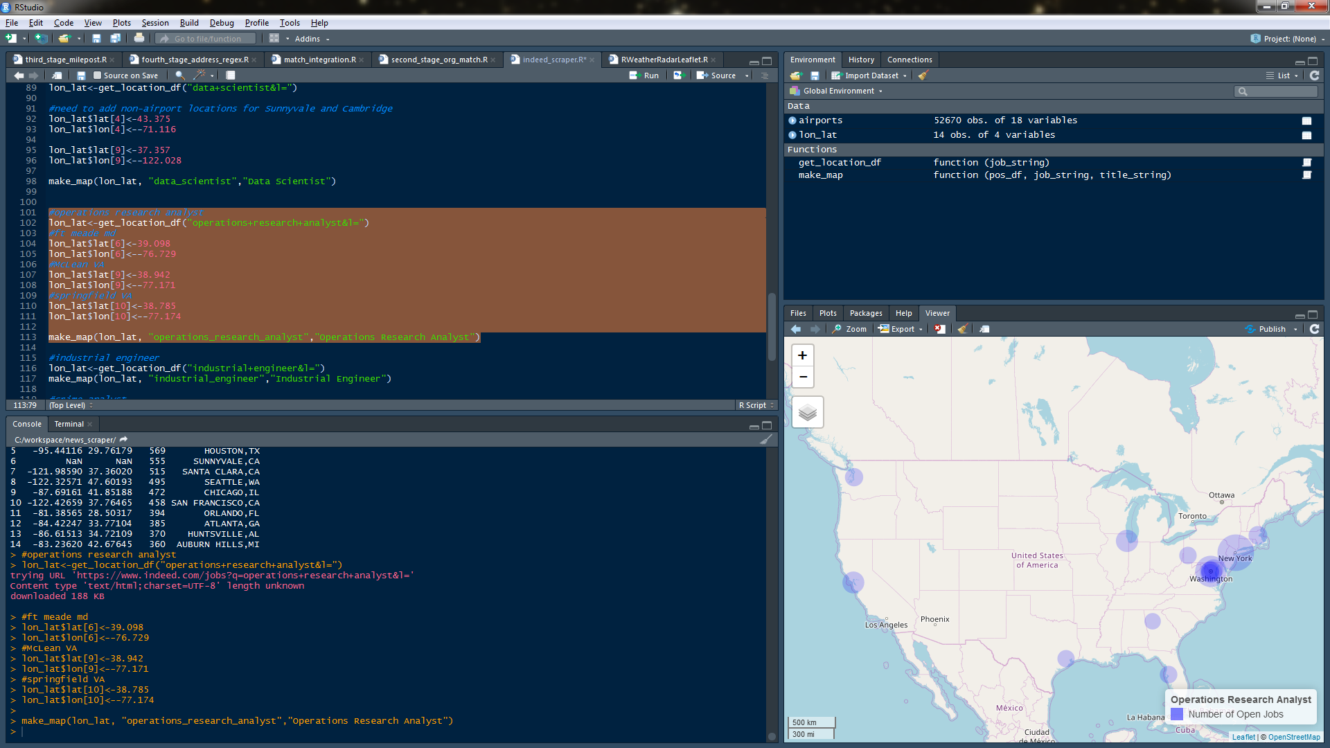
Now I’ll call my map function:
make_map(lon_lat, "operations_research_analyst","Operations Research Analyst")
And I should see my map in RStudio:
Or if I go to the html page on my hard drive:
I don’t have much to offer in the way of commentary on the location of these positions, except to say they’re weren’t too many surprises. Here are the interactive maps I made with the script.
https://enholm.net/maps/operations_research_analyst.html
https://enholm.net/maps/data_scientist.html
https://enholm.net/maps/industrial_engineer.html
https://enholm.net/maps/crime_analyst.html


